Run this tutorial: Open in Colab | Launch Binder

EnbPI prediction intervals and the four calibrators

A point forecast tells you nothing about how wrong it might be. EnbPI wraps an ordinary sklearn regressor in prediction intervals, and four calibrators turn one set of residuals into widths. We build the intervals, line the calibrators up, and watch how each behaves when volatility clusters.

EnbPI (Xu and Xie 2021) works like this. Fit the regressor on each bootstrap resample of the rows, predict the rows that were left out, and collect the out-of-bag absolute residuals. The (1 - alpha) quantile of those residuals is a half-width: center an interval on the prediction, add and subtract the half-width. The bootstrap ensemble is the only machinery; the regressor itself never has to know about uncertainty.

A caveat to keep in mind throughout. EnbPI coverage is approximate and asymptotic under temporal dependence (a strong-mixing condition), not finite-sample distribution-free like split conformal on exchangeable data. The intervals target marginal (1 - alpha) coverage averaged over time; they do not promise it at every point, and under distribution shift the base method can drift off target. The adaptive calibrators below exist to fight that drift, and each carries a different guarantee that we label as we go.

The plan:

1. Build a regression-from-lags problem from a time series.

2. Fit EnbPIEnsemble once with a moving-block bootstrap.

3. Read intervals out under all four calibrators: static, sliding window, ACI, NexCP.

4. Judge them with the canonical interval-quality plots and the Winkler score.

5. Stress them on a GARCH-style volatility-clustering series where static breaks.

# On Colab or Binder, install tsbootstrap first (skipped if already present):
try:
    import tsbootstrap  # noqa: F401
except ImportError:
    %pip install -q "tsbootstrap[examples]"

Inline data-generating processes and helpers

Two inline DGPs, a lag-feature builder, and the interval-quality metrics. We use two series with known structure:

• AR(2), x[t] = 0.6 x[t-1] - 0.3 x[t-2] + e[t], homoskedastic. A regression on the two previous values is correctly specified, so this is the easy baseline where even the static calibrator should do well.

• GARCH(1,1)-style, a conditionally heteroskedastic series whose variance clusters: calm stretches and turbulent stretches alternate. The conditional mean is still a mild AR(1), but the noise scale moves over time. This is where a single global width is wrong by construction, and the time-local and drift-adaptive calibrators should earn their keep.

import matplotlib.pyplot as plt
import numpy as np
import pandas as pd
from sklearn.linear_model import LinearRegression

from tsbootstrap import MovingBlock
from tsbootstrap.uq import EnbPIEnsemble

# Colorblind-safe per-calibrator style: each calibrator is distinguished by line
# style AND marker (and hatch for bars), not by color alone, so the plots stay
# legible in grayscale and for color-vision-deficient readers.
CALIB_STYLE = {
    "static": {"color": "#0072B2", "ls": "-", "marker": "o", "hatch": "//"},
    "sliding_window": {"color": "#E69F00", "ls": "--", "marker": "s", "hatch": ".."},
    "aci": {"color": "#009E73", "ls": "-.", "marker": "^", "hatch": "xx"},
    "nexcp": {"color": "#D55E00", "ls": ":", "marker": "D", "hatch": "\\\\"},
}
CALIB_LABEL = {
    "static": "static",
    "sliding_window": "sliding window",
    "aci": "ACI",
    "nexcp": "NexCP",
}


def ar2(n, phi1=0.6, phi2=-0.3, rng=None):
    """Stationary AR(2), unit-variance Gaussian noise, started at 0."""
    rng = np.random.default_rng() if rng is None else rng
    x = np.zeros(n)
    e = rng.standard_normal(n)
    for t in range(2, n):
        x[t] = phi1 * x[t - 1] + phi2 * x[t - 2] + e[t]
    return x


def garch11(n, omega=0.05, alpha=0.12, beta=0.85, ar=0.3, rng=None, burn=200):
    """AR(1) mean with GARCH(1,1) conditional variance: volatility clusters over time.

    sigma2_t = omega + alpha * eps_{t-1}**2 + beta * sigma2_{t-1}, eps_t = sigma_t z_t,
    x_t = ar * x_{t-1} + eps_t. alpha + beta < 1 keeps it stationary.
    """
    rng = np.random.default_rng() if rng is None else rng
    total = n + burn
    z = rng.standard_normal(total)
    sigma2 = np.empty(total)
    eps = np.empty(total)
    x = np.zeros(total)
    sigma2[0] = omega / max(1e-8, 1 - alpha - beta)
    eps[0] = np.sqrt(sigma2[0]) * z[0]
    for t in range(1, total):
        sigma2[t] = omega + alpha * eps[t - 1] ** 2 + beta * sigma2[t - 1]
        eps[t] = np.sqrt(sigma2[t]) * z[t]
        x[t] = ar * x[t - 1] + eps[t]
    return x[burn:], np.sqrt(sigma2[burn:])


def lag_design(series, n_lags):
    """Build (X, y) for a regression from the last n_lags values onto the next value.

    X[i] = [s[i + n_lags - 1], ..., s[i]] (most-recent lag first), y[i] = s[i + n_lags].
    Returns X of shape (len - n_lags, n_lags) and y of shape (len - n_lags,), time-aligned.
    """
    s = np.asarray(series, dtype=float)
    n = s.shape[0]
    n - n_lags
    X = np.column_stack([s[n_lags - 1 - k : n - 1 - k] for k in range(n_lags)])
    y = s[n_lags:]
    return X, y, np.arange(n_lags, n)  # third item: the time index of each target


def empirical_coverage(lo, hi, y):
    """Fraction of targets inside [lo, hi]."""
    return float(np.mean((y >= lo) & (y <= hi)))


def running_coverage(lo, hi, y):
    """Cumulative coverage up to each time t (a running average of the hit indicator)."""
    hit = ((y >= lo) & (y <= hi)).astype(float)
    return np.cumsum(hit) / np.arange(1, hit.size + 1)


def winkler_score(lo, hi, y, alpha):
    """Mean Winkler interval score (lower is better).

    width + (2 / alpha) * (lo - y) if y < lo, + (2 / alpha) * (y - hi) if y > hi, else 0.
    Rewards narrow intervals but penalizes misses in proportion to how far outside they fall.
    """
    width = hi - lo
    below = np.maximum(lo - y, 0.0)
    above = np.maximum(y - hi, 0.0)
    return float(np.mean(width + (2.0 / alpha) * (below + above)))

A regression-from-lags problem

We turn forecasting into tabular regression: predict the next value from the two previous ones. That makes the model an ordinary LinearRegression, and lets the out-of-bag bootstrap supply held-out residuals for every row.

EnbPI needs an observation-resampling method so each replicate has a real out-of-bag set. We use MovingBlock, which resamples contiguous blocks of rows and so respects local dependence in the residuals. (A recursive model method has no row indices and would be rejected.) We keep n_bootstraps modest at 80.

N_LAGS = 2
ALPHA = 0.1  # target 90% intervals
N_BOOTSTRAPS = 80
BLOCK = 12

rng = np.random.default_rng(0)
x_ar2 = ar2(700, rng=rng)
X, y, t_idx = lag_design(x_ar2, N_LAGS)
print(f"design matrix {X.shape}, targets {y.shape}")

ens = EnbPIEnsemble().fit(
    LinearRegression(),
    X,
    y,
    method=MovingBlock(block_length=BLOCK),
    n_bootstraps=N_BOOTSTRAPS,
    random_state=1,
)
print(f"out-of-bag residuals collected: {ens.oob_residuals.shape[0]}")
print(f"median |oob residual| = {np.median(ens.oob_residuals):.3f}")

design matrix (698, 2), targets (698,)
out-of-bag residuals collected: 698
median |oob residual| = 0.682

All four calibrators from one fit

The ensemble is fitted once. Each calibrator is just a different reading of the same out-of-bag residual buffer, passed at predict time:

• static: one global (1 - alpha) quantile, the same width everywhere. Original EnbPI. Guarantee: approximate marginal (1 - alpha) coverage, averaged over time.

• sliding_window: a rolling (1 - alpha) quantile over a trailing window, so the width tracks local volatility. Guarantee: still approximate marginal, but adapts to changing scale (time-local EnbPI).

• aci (Adaptive Conformal Inference, Gibbs and Candes 2021): adjusts the quantile level online from realized coverage errors. Needs the realized test scores |y_t - prediction_t| in time order. Guarantee: long-run time-average coverage converges to 1 - alpha even under arbitrary distribution shift; it does not promise marginal coverage at any single step.

• nexcp (Nonexchangeable Conformal Prediction, Barber et al. 2023): a recency-weighted quantile via a decay. Guarantee: a finite-sample coverage bound minus a drift gap that grows with how fast the distribution moves; with decay = 1 it is the ordinary quantile.

For ACI the realized scores are the in-sample |y - point|; we compute them from the static point prediction (the out-of-bag ensemble mean, identical across calibrators).

lo_s, hi_s, point = ens.predict_interval(alpha=ALPHA, calibrator="static")

# Realized non-conformity scores for ACI: one per prediction row, in time order.
test_scores = np.abs(y - point)

intervals = {}
intervals["static"] = (lo_s, hi_s)
intervals["sliding_window"] = ens.predict_interval(
    alpha=ALPHA, calibrator="sliding_window", window=60
)[:2]
intervals["aci"] = ens.predict_interval(
    alpha=ALPHA, calibrator="aci", test_scores=test_scores, gamma=0.05
)[:2]
intervals["nexcp"] = ens.predict_interval(alpha=ALPHA, calibrator="nexcp", decay=0.97)[:2]

guarantee = {
    "static": "approx. marginal (EnbPI)",
    "sliding_window": "approx. marginal, time-local",
    "aci": "long-run time-average, shift-robust",
    "nexcp": "finite-sample minus drift gap",
}

ar2_summary = pd.DataFrame(
    {
        CALIB_LABEL[name]: {
            "coverage": empirical_coverage(lo, hi, y),
            "mean width": float(np.mean(hi - lo)),
            "Winkler": winkler_score(lo, hi, y, ALPHA),
            "guarantee": guarantee[name],
        }
        for name, (lo, hi) in intervals.items()
    }
).T
print(f"AR(2) baseline, nominal coverage = {1 - ALPHA:.0%}:")
ar2_summary

AR(2) baseline, nominal coverage = 90%:

	coverage	mean width	Winkler	guarantee
static	0.899713	3.068552	4.102011	approx. marginal (EnbPI)
sliding window	0.891117	3.068784	4.056283	approx. marginal, time-local
ACI	0.899713	3.299156	4.252896	long-run time-average, shift-robust
NexCP	0.886819	2.982549	4.10815	finite-sample minus drift gap

On the homoskedastic AR(2) the four calibrators land close together: the scale is constant, so there is little for the adaptive ones to adapt to. They all sit near the nominal 90% line, and the Winkler scores are within a hair of each other. The real separation appears once volatility moves, which is the next section. First, the canonical interval-quality views on this baseline.

Interval-quality plot 1: the interval over time, with misses highlighted

Start with the interval itself: the realized series threading through a band, with the points that fall outside marked. We show a 200-step window of the static-calibrator band so the structure is legible.

lo, hi = intervals["static"]
sl = slice(150, 350)
tt = t_idx[sl]
miss = (y[sl] < lo[sl]) | (y[sl] > hi[sl])

fig, ax = plt.subplots(figsize=(10, 4), layout="constrained")
ax.fill_between(
    tt, lo[sl], hi[sl], color="#0072B2", alpha=0.20, label=f"static {1 - ALPHA:.0%} interval"
)
ax.plot(tt, point[sl], color="#0072B2", lw=1.0, label="point prediction")
ax.plot(tt, y[sl], color="black", lw=1.0, label="realized value")
ax.scatter(
    tt[miss],
    y[sl][miss],
    color="#D55E00",
    marker="X",
    s=55,
    edgecolor="black",
    linewidth=0.5,
    zorder=5,
    label="realized point outside band",
)
ax.set_title("EnbPI static prediction interval over time (AR(2) series)")
ax.set_xlabel("time index (steps)")
ax.set_ylabel("series value (unitless)")
ax.legend(loc="upper right", fontsize=8, framealpha=0.9)
plt.show()

print(f"misses in window: {int(miss.sum())} / {miss.size} ({miss.mean():.1%}; target {ALPHA:.0%})")

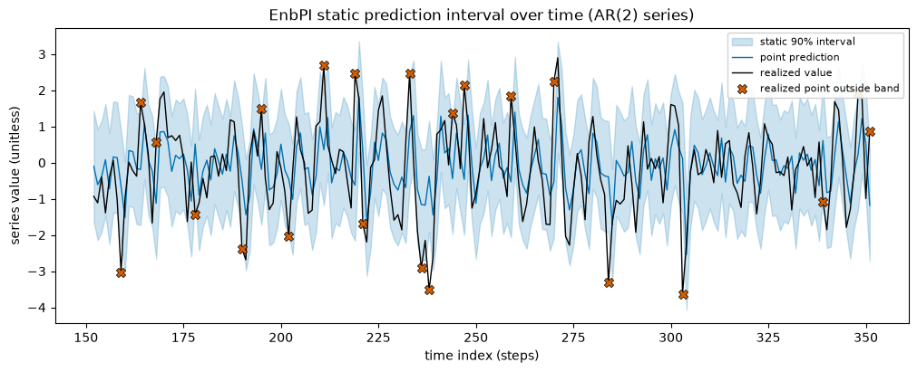
misses in window: 22 / 200 (11.0%; target 10%)

The realized series mostly stays inside the band, with a sprinkling of red misses at roughly the target rate. On a constant-variance process a constant-width band is the right shape, so this looks healthy.

Interval-quality plot 2: running coverage versus the nominal line

A single coverage number hides when the misses happen. The running (cumulative) coverage shows whether the interval is on target throughout, or only on average because an early over-cover cancels a late under-cover. A well-calibrated interval hugs the nominal line.

fig, ax = plt.subplots(figsize=(10, 4.5), layout="constrained")
for name, (lo, hi) in intervals.items():
    st = CALIB_STYLE[name]
    ax.plot(
        t_idx,
        running_coverage(lo, hi, y),
        color=st["color"],
        ls=st["ls"],
        marker=st["marker"],
        markevery=80,
        markersize=5,
        lw=1.4,
        label=CALIB_LABEL[name],
    )
ax.axhline(
    1 - ALPHA, color="black", ls=(0, (6, 4)), lw=1.4, label=f"nominal {1 - ALPHA:.0%} coverage"
)
ax.set_ylim(0.6, 1.0)
ax.set_title("Running coverage vs nominal target (AR(2) series)")
ax.set_xlabel("time index (steps)")
ax.set_ylabel("cumulative coverage (fraction)")
ax.legend(fontsize=8, loc="lower right", ncol=2, framealpha=0.9)
plt.show()

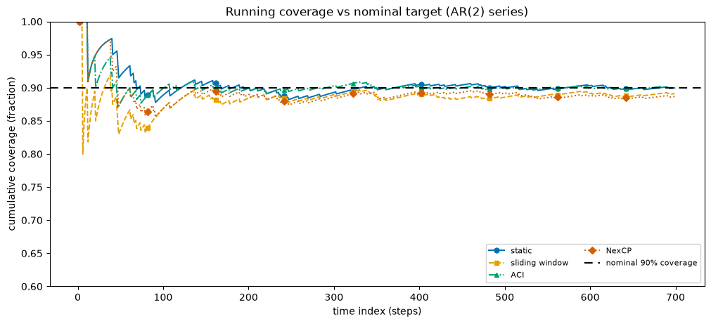
All four curves settle near the dashed nominal line, after the usual noisy start where only a few points have been seen. On the easy series, the calibrators are interchangeable; this plot is the diagnostic that will separate them on the GARCH series below.

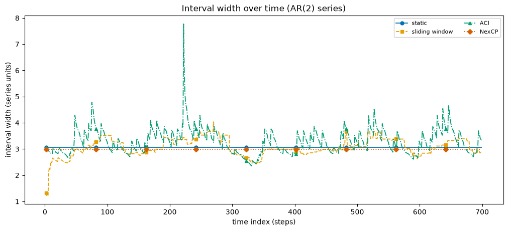
Interval-quality plot 3: interval width over time

Coverage alone is not enough: a band that covers only by being enormous is useless. The width-over-time view shows how each calibrator spends its budget. On a homoskedastic series the static and NexCP widths are flat; the sliding window wobbles slightly with local residual noise; ACI breathes as it chases realized coverage.

fig, ax = plt.subplots(figsize=(10, 4.5), layout="constrained")
for name, (lo, hi) in intervals.items():
    st = CALIB_STYLE[name]
    ax.plot(
        t_idx,
        hi - lo,
        color=st["color"],
        ls=st["ls"],
        marker=st["marker"],
        markevery=80,
        markersize=5,
        lw=1.3,
        label=CALIB_LABEL[name],
    )
ax.set_title("Interval width over time (AR(2) series)")
ax.set_xlabel("time index (steps)")
ax.set_ylabel("interval width (series units)")
ax.legend(fontsize=8, loc="upper right", ncol=2, framealpha=0.9)
plt.show()

Interval-quality plot 4: coverage versus target as alpha sweeps

A calibration line sweeps the target coverage and plots achieved against requested. The diagonal is perfect calibration. A curve below the diagonal under-covers (too narrow); above it over-covers (too wide). We sweep the static calibrator since it has the cleanest single quantile interpretation.

targets = np.linspace(0.5, 0.95, 10)
achieved = []
for tgt in targets:
    a = 1 - tgt
    lo, hi, _ = ens.predict_interval(alpha=a, calibrator="static")
    achieved.append(empirical_coverage(lo, hi, y))
achieved = np.array(achieved)

fig, ax = plt.subplots(figsize=(6, 6), layout="constrained")
ax.plot(
    [0.5, 1.0],
    [0.5, 1.0],
    color="black",
    ls=(0, (6, 4)),
    lw=1.4,
    label="perfect calibration (y = x)",
)
ax.plot(targets, achieved, ls="-", marker="o", markersize=6, color="#0072B2", label="EnbPI static")
ax.set_xlabel("target coverage 1 - alpha (fraction)")
ax.set_ylabel("achieved in-sample coverage (fraction)")
ax.set_title("Calibration line: achieved vs requested coverage (AR(2) series)")
ax.legend(loc="upper left", fontsize=9, framealpha=0.9)
ax.set_aspect("equal")
plt.show()

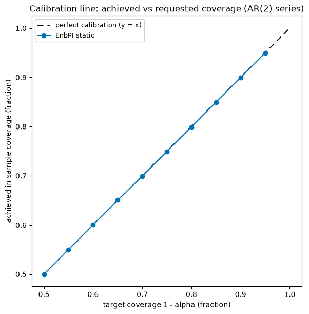
The static calibrator tracks the diagonal closely on the AR(2): asking for x% coverage returns about x%. That is the best case, a correctly specified model on a constant-variance series. The GARCH stress test breaks this for the static method and shows which calibrators repair it.

The stress test: a GARCH(1,1) volatility-clustering series

Now the hard case. The GARCH series has stretches of calm and stretches of turbulence. A single global width is too wide in the calm stretches (wasting tightness) and too narrow in the turbulent ones (missing exactly when it matters most). This is where the time-local and drift-adaptive calibrators are supposed to pull ahead.

Two calibrator knobs need a gentler setting here than on the calm baseline. ACI’s gamma is its step size: a large step on a volatile series can drive the adapted level past zero, at which point ACI deliberately returns an infinite half-width to “cover everything” until it recovers. We use a smaller gamma = 0.02 so the level stays in range and the widths stay finite. NexCP’s decay controls how fast old residuals are forgotten; an aggressive decay over-reacts to a turbulent stretch and over-covers, so we soften it to decay = 0.995.

rng_g = np.random.default_rng(7)
x_garch, sigma_true = garch11(900, rng=rng_g)
Xg, yg, tg = lag_design(x_garch, N_LAGS)
sigma_y = sigma_true[N_LAGS:]  # conditional sd aligned to the targets

ens_g = EnbPIEnsemble().fit(
    LinearRegression(),
    Xg,
    yg,
    method=MovingBlock(block_length=BLOCK),
    n_bootstraps=N_BOOTSTRAPS,
    random_state=2,
)

lo_g, hi_g, point_g = ens_g.predict_interval(alpha=ALPHA, calibrator="static")
test_scores_g = np.abs(yg - point_g)

intervals_g = {}
intervals_g["static"] = (lo_g, hi_g)
intervals_g["sliding_window"] = ens_g.predict_interval(
    alpha=ALPHA, calibrator="sliding_window", window=60
)[:2]
intervals_g["aci"] = ens_g.predict_interval(
    alpha=ALPHA, calibrator="aci", test_scores=test_scores_g, gamma=0.02
)[:2]
intervals_g["nexcp"] = ens_g.predict_interval(alpha=ALPHA, calibrator="nexcp", decay=0.995)[:2]

garch_summary = pd.DataFrame(
    {
        CALIB_LABEL[name]: {
            "coverage": empirical_coverage(lo, hi, yg),
            "mean width": float(np.mean(hi - lo)),
            "Winkler": winkler_score(lo, hi, yg, ALPHA),
            "guarantee": guarantee[name],
        }
        for name, (lo, hi) in intervals_g.items()
    }
).T
print(f"GARCH(1,1) stress test, nominal coverage = {1 - ALPHA:.0%}:")
garch_summary

GARCH(1,1) stress test, nominal coverage = 90%:

	coverage	mean width	Winkler	guarantee
static	0.899777	3.523932	4.417807	approx. marginal (EnbPI)
sliding window	0.885301	3.327023	4.266725	approx. marginal, time-local
ACI	0.894209	3.465232	4.400078	long-run time-average, shift-robust
NexCP	0.927617	3.807192	4.453241	finite-sample minus drift gap

GARCH plot: width tracking the true conditional volatility

The defining test of a time-local interval is whether its width follows the true volatility. We overlay each calibrator’s width on a scaled copy of the true GARCH conditional standard deviation. The sliding window should track the volatility ridge; the static width is a flat line that cannot.

sl = slice(0, 500)
ts = tg[sl]
# Scale the true sd to the static width band for visual comparison of *shape*.
sigma_plot = (
    sigma_y[sl] / sigma_y.mean() * np.mean(intervals_g["static"][1] - intervals_g["static"][0])
)

fig, ax = plt.subplots(figsize=(10, 4.5), layout="constrained")
ax.plot(ts, sigma_plot, color="gray", lw=2.5, alpha=0.7, label="true conditional sd (scaled)")
for name in ["static", "sliding_window", "nexcp"]:
    lo, hi = intervals_g[name]
    st = CALIB_STYLE[name]
    ax.plot(
        ts,
        (hi - lo)[sl],
        color=st["color"],
        ls=st["ls"],
        marker=st["marker"],
        markevery=50,
        markersize=5,
        lw=1.4,
        label=f"{CALIB_LABEL[name]} width",
    )
ax.set_title("Interval width vs true conditional volatility (GARCH series)")
ax.set_xlabel("time index (steps)")
ax.set_ylabel("interval width / scaled volatility (series units)")
ax.legend(fontsize=8, loc="upper right", ncol=2, framealpha=0.9)
plt.show()

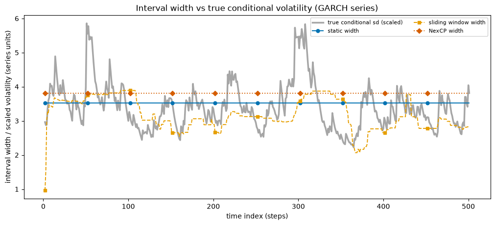
The static width is a flat line, blind to the volatility ridge under it. The sliding-window width rises and falls with the true conditional standard deviation: wider when the series is turbulent, tighter when it is calm. That is the whole point of a time-local interval, and it is why the sliding window covers the dangerous high-volatility stretches that a fixed width misses.

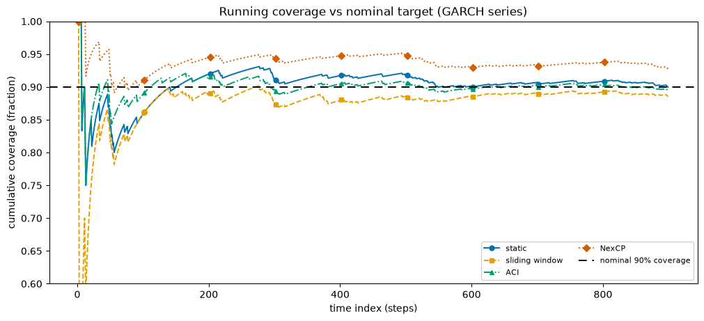
GARCH plot: running coverage separates the calibrators

On the GARCH series the running-coverage plot finally pulls the calibrators apart. The static line dips during turbulent stretches (its fixed width is too narrow there); the adaptive calibrators hold closer to nominal because they widen when volatility rises.

fig, ax = plt.subplots(figsize=(10, 4.5), layout="constrained")
for name, (lo, hi) in intervals_g.items():
    st = CALIB_STYLE[name]
    ax.plot(
        tg,
        running_coverage(lo, hi, yg),
        color=st["color"],
        ls=st["ls"],
        marker=st["marker"],
        markevery=100,
        markersize=5,
        lw=1.4,
        label=CALIB_LABEL[name],
    )
ax.axhline(
    1 - ALPHA, color="black", ls=(0, (6, 4)), lw=1.4, label=f"nominal {1 - ALPHA:.0%} coverage"
)
ax.set_ylim(0.6, 1.0)
ax.set_title("Running coverage vs nominal target (GARCH series)")
ax.set_xlabel("time index (steps)")
ax.set_ylabel("cumulative coverage (fraction)")
ax.legend(fontsize=8, loc="lower right", ncol=2, framealpha=0.9)
plt.show()

Interval-quality plot 5: conditional coverage by volatility bin

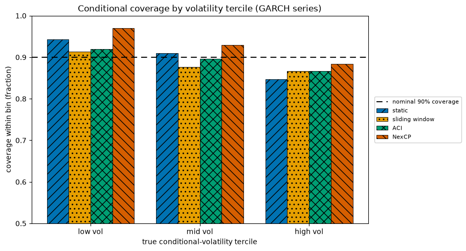
Marginal coverage can be exactly right while conditional coverage is badly wrong: an interval can over-cover calm periods and under-cover turbulent ones, averaging out to the nominal rate while failing precisely when you need it. We bin the GARCH targets by their true conditional volatility (terciles) and measure coverage within each bin. A flat profile near nominal is the goal; a downward slope from calm to turbulent bins is the failure a fixed width makes.

edges = np.quantile(sigma_y, [0.0, 1 / 3, 2 / 3, 1.0])
bin_idx = np.clip(np.digitize(sigma_y, edges[1:-1]), 0, 2)
bin_labels = ["low vol", "mid vol", "high vol"]

# Coverage within each volatility bin, per calibrator.
cond_cov = {}
for name, (lo, hi) in intervals_g.items():
    hit = ((yg >= lo) & (yg <= hi)).astype(float)
    cond_cov[name] = [hit[bin_idx == b].mean() for b in range(3)]

fig, ax = plt.subplots(figsize=(9, 4.8), layout="constrained")
bar_w = 0.2
xpos = np.arange(3)
for j, name in enumerate(intervals_g):
    st = CALIB_STYLE[name]
    ax.bar(
        xpos + (j - 1.5) * bar_w,
        cond_cov[name],
        bar_w,
        color=st["color"],
        hatch=st["hatch"],
        edgecolor="black",
        linewidth=0.6,
        label=CALIB_LABEL[name],
    )
ax.axhline(
    1 - ALPHA, color="black", ls=(0, (6, 4)), lw=1.4, label=f"nominal {1 - ALPHA:.0%} coverage"
)
ax.set_xticks(xpos)
ax.set_xticklabels(bin_labels)
ax.set_ylim(0.5, 1.0)
ax.set_xlabel("true conditional-volatility tercile")
ax.set_ylabel("coverage within bin (fraction)")
ax.set_title("Conditional coverage by volatility tercile (GARCH series)")
ax.legend(fontsize=8, loc="center left", bbox_to_anchor=(1.01, 0.5), framealpha=0.9)
plt.show()

cond_table = pd.DataFrame(
    {CALIB_LABEL[name]: cond_cov[name] for name in intervals_g},
    index=bin_labels,
).T
cond_table.columns.name = "volatility bin"
print(f"Conditional coverage by volatility tercile (target = {1 - ALPHA:.0%}):")
cond_table.round(3)

Conditional coverage by volatility tercile (target = 90%):

volatility bin	low vol	mid vol	high vol
static	0.943	0.910	0.847
sliding window	0.913	0.876	0.867
ACI	0.920	0.896	0.867
NexCP	0.970	0.930	0.883

The static calibrator’s bars slope down: it over-covers the low-volatility bin (wasted width) and under-covers the high-volatility bin (the dangerous failure), even when its marginal number looked acceptable. The sliding-window and NexCP bars are flatter, because their widths grow in the turbulent bin. That flattening is the conditional-coverage repair a fixed width cannot provide.

Winkler scores: one number to compare calibrators

The Winkler interval score combines width and miss penalty into a single number (lower is better): you pay the interval width always, plus 2 / alpha times how far any realized point falls outside. It rewards tight intervals but punishes a miss far more than it rewards the narrowness that caused it, so it cannot be gamed by shrinking the band. We compare all four calibrators on both series.

def winkler_frame(intervals_map, y):
    """Coverage, mean width and Winkler score per calibrator, as a DataFrame."""
    rows = {}
    for name, (lo, hi) in intervals_map.items():
        rows[CALIB_LABEL[name]] = {
            "coverage": empirical_coverage(lo, hi, y),
            "mean width": float(np.mean(hi - lo)),
            "Winkler": winkler_score(lo, hi, y, ALPHA),
        }
    return pd.DataFrame(rows).T


ar2_table = winkler_frame(intervals, y)
garch_table = winkler_frame(intervals_g, yg)

comparison = pd.concat(
    {"AR(2) homoskedastic": ar2_table, "GARCH(1,1) clustering": garch_table},
    names=["series", "calibrator"],
)
print(
    f"Interval quality on both series (nominal coverage = {1 - ALPHA:.0%}; "
    "lower Winkler is better):"
)
print("AR(2) best Winkler:  ", ar2_table["Winkler"].idxmin())
print("GARCH best Winkler:  ", garch_table["Winkler"].idxmin())
comparison.round(3)

Interval quality on both series (nominal coverage = 90%; lower Winkler is better):
AR(2) best Winkler:   sliding window
GARCH best Winkler:   sliding window

		coverage	mean width	Winkler
series	calibrator
AR(2) homoskedastic	static	0.900	3.069	4.102
	sliding window	0.891	3.069	4.056
	ACI	0.900	3.299	4.253
	NexCP	0.887	2.983	4.108
GARCH(1,1) clustering	static	0.900	3.524	4.418
	sliding window	0.885	3.327	4.267
	ACI	0.894	3.465	4.400
	NexCP	0.928	3.807	4.453

What to take away

EnbPI gives any sklearn regressor a prediction interval from nothing more than its own out-of-bag residuals, and the calibrator chooses how those residuals become a width.

• On a homoskedastic series (AR(2)) all four calibrators are close: there is no drifting scale to adapt to, so the simple static width is already near optimal on both coverage and Winkler score.

• On a heteroskedastic series (GARCH) the static calibrator fails conditionally: it under-covers the high-volatility stretches that matter most, even when its marginal coverage looks fine. The time-local sliding window and the recency-weighted NexCP widen with the volatility and flatten the conditional-coverage profile; ACI holds long-run coverage by adjusting its level online.

Match the guarantee to your problem. Static is the default under stable conditions, where its approximate marginal coverage is all you need. Sliding window is the upgrade when the noise scale moves. ACI is the choice under genuine distribution shift, where its long-run time-average guarantee is robust by construction. NexCP buys a finite-sample bound at the cost of a drift gap that grows with how fast the world changes. All of them stay approximate or asymptotic under temporal dependence rather than finite-sample distribution-free, which is the ceiling for time-series uncertainty.