Run this tutorial: Open in Colab | Launch Binder

sktime / skbase adapters: bootstraps as estimator classes

Every method in tsbootstrap is reachable two ways. The quickstart used the functional core: one bootstrap() call configured with a typed spec. This notebook uses the object-oriented surface. Under tsbootstrap.adapters each method is also a skbase.BaseObject estimator class with a scikit-learn style constructor and a .bootstrap(...) generator.

Both surfaces exist for different reasons. The functional core stays stateless and easy to accelerate. The adapter classes carry parameters, support get_params / set_params / clone, and expose sktime tags, so they drop into sktime pipelines and the skbase object registry. The algorithms are the same; the two surfaces differ only in how you reach them. What follows lists the adapter classes, runs a few on the bundled airline dataset, shows the return_indices behavior, reads the sktime tags, and checks the skbase object contract.

# On Colab or Binder, install tsbootstrap first (skipped if already present):
try:
    import tsbootstrap  # noqa: F401
except ImportError:
    %pip install -q "tsbootstrap[examples]"

The adapter classes

The adapters live in tsbootstrap.adapters. Each one wraps a method from the functional core as a thin estimator. Here is the full set that ships, read off the package, with the sktime tags each carries.

import pandas as pd

import tsbootstrap.adapters as adapters

rows = []
for name in adapters.__all__:
    if name == "BaseTimeSeriesBootstrap":
        continue  # the shared base, not a concrete method
    cls = getattr(adapters, name)
    tags = cls.get_class_tags()
    rows.append(
        {
            "adapter": name,
            "bootstrap_type": tags["bootstrap_type"],
            "multivariate": tags["capability:multivariate"],
        }
    )

adapter_table = pd.DataFrame(rows).set_index("adapter")
adapter_table

	bootstrap_type	multivariate
adapter
IIDBootstrap	iid	True
MovingBlockBootstrap	block	True
CircularBlockBootstrap	block	True
StationaryBlockBootstrap	block	True
NonOverlappingBlockBootstrap	block	True
TaperedBlockBootstrap	block	True
ARResidualBootstrap	model	False
ARIMAResidualBootstrap	model	False
VARResidualBootstrap	model	True
SieveBootstrap	model	False

The columns mirror the functional taxonomy: iid resampling, block methods (moving, circular, stationary, non-overlapping, tapered), and model based bootstraps (AR, ARIMA, VAR residual, and the sieve). BaseTimeSeriesBootstrap is the shared base that holds the delegation logic; it is not a method you instantiate directly.

The data: airline passengers

We use the classic monthly airline passenger counts bundled with sktime. It is small (144 points), real, and has both trend and seasonality, so the different bootstrap families behave visibly differently on it.

import matplotlib.pyplot as plt
import numpy as np
from sktime.datasets import load_airline

y = load_airline()
print("type:", type(y).__name__, " length:", len(y))
y_values = y.to_numpy(dtype=float)
y_values[:6]

type: Series  length: 144

array([112., 118., 132., 129., 121., 135.])

Constructing an estimator and running its generator

The constructor takes the method’s parameters plus n_bootstraps and random_state, scikit-learn style. Calling .bootstrap(X) returns a generator that yields n_bootstraps replicate series. We pass the raw NumPy values; each yielded replicate is a NumPy array the same length as the input.

from tsbootstrap.adapters import MovingBlockBootstrap

mbb = MovingBlockBootstrap(block_length=12, n_bootstraps=200, random_state=0)
print("get_params:", mbb.get_params())
print("get_n_bootstraps:", mbb.get_n_bootstraps())

gen = mbb.bootstrap(y_values)  # a generator, nothing computed yet
import types

print("is a generator:", isinstance(gen, types.GeneratorType))

replicates = list(gen)  # draining the generator does the work
print("collected:", len(replicates), "replicates, each shape", replicates[0].shape)

get_params: {'block_length': 12, 'n_bootstraps': 200, 'random_state': 0}
get_n_bootstraps: 200
is a generator: True
collected: 200 replicates, each shape (144,)

Three adapters end to end

We run three different families on the airline series and overlay eight replicates from each on a single plot: the moving block (keeps local seasonal runs), the i.i.d. baseline (shuffles all structure away), and the AR residual bootstrap (resamples innovations around a fitted AR model). Each family gets its own colour and linestyle so they stay distinguishable in grayscale. The differences between them are why you would pick one method over another.

from tsbootstrap.adapters import ARResidualBootstrap, IIDBootstrap

estimators = {
    "MovingBlockBootstrap(block_length=12)": MovingBlockBootstrap(
        block_length=12, n_bootstraps=50, random_state=0
    ),
    "IIDBootstrap()": IIDBootstrap(n_bootstraps=50, random_state=0),
    "ARResidualBootstrap(order=2)": ARResidualBootstrap(order=2, n_bootstraps=50, random_state=0),
}

# Colorblind-safe palette (Wong 2011); each adapter also gets a distinct
# linestyle so the families stay distinguishable in grayscale or for readers
# with colour-vision deficiency.
styles = {
    "MovingBlockBootstrap(block_length=12)": ("#0072B2", "-"),  # blue, solid
    "IIDBootstrap()": ("#E69F00", "--"),  # orange, dashed
    "ARResidualBootstrap(order=2)": ("#009E73", ":"),  # green, dotted
}

months = np.arange(1, len(y_values) + 1)

fig, ax = plt.subplots(figsize=(9, 5), layout="constrained")

# Faint replicate clouds, eight per adapter, coloured + styled per family.
for label, est in estimators.items():
    color, ls = styles[label]
    for i, rep in enumerate(est.bootstrap(y_values)):
        if i >= 8:
            break
        ax.plot(months, rep, color=color, linestyle=ls, alpha=0.35, lw=0.9, zorder=1)

# Original series emphasized on top, in front of every replicate.
ax.plot(months, y_values, color="black", lw=2.6, zorder=3, label="Original airline series")

# One bold proxy line per adapter for a readable legend (the faint replicates
# would otherwise make the legend swatches nearly invisible).
from matplotlib.lines import Line2D

legend_handles = [Line2D([0], [0], color="black", lw=2.6, label="Original airline series")]
legend_handles += [
    Line2D([0], [0], color=styles[label][0], linestyle=styles[label][1], lw=2.0, label=label)
    for label in estimators
]

ax.set_title("Eight bootstrap replicates per adapter family, overlaid on the airline series")
ax.set_xlabel("Time (months from start of series)")
ax.set_ylabel("Air passengers (thousands)")
ax.set_xlim(months[0], months[-1])
ax.legend(handles=legend_handles, loc="upper left", framealpha=0.9, fontsize=9)
ax.grid(True, alpha=0.25, linewidth=0.5)
plt.show()

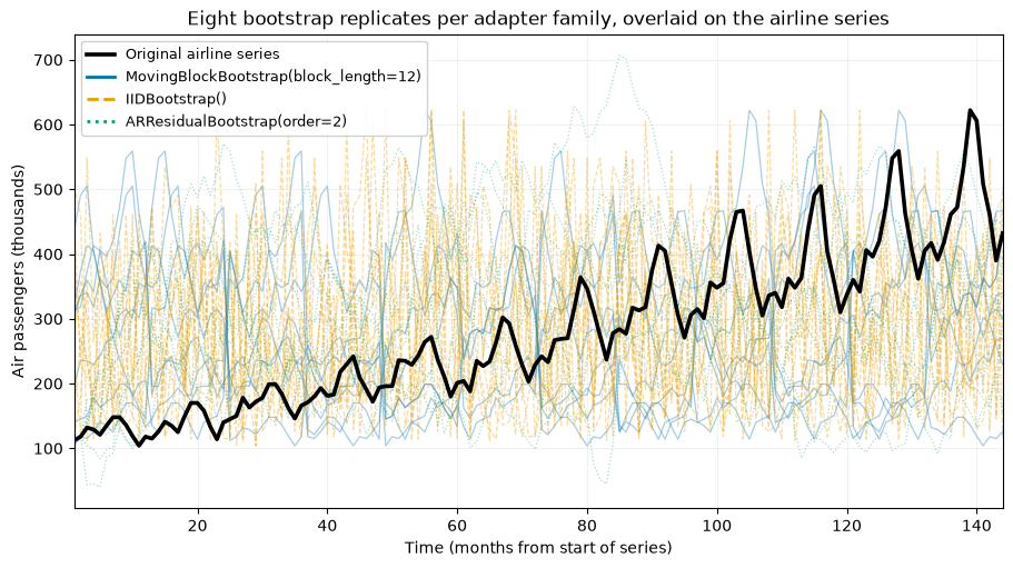
The moving block replicates (blue, solid) preserve stretches of the original seasonal shape, just reshuffled in time. The IID replicates (orange, dashed) lose that ordering, so the trend and seasonality collapse into noise around the level. The AR residual replicates (green, dotted) keep a smooth autoregressive character because they rebuild each series from a fitted model and resampled innovations. The overlay shows how much each method’s assumptions change what a replicate looks like.

return_indices: where each value came from

By default the generator yields just the replicate series. Pass return_indices=True and it yields (sample, indices) pairs instead, where indices are the positions in the original series that were drawn (or None for methods that do not resample observations). This is what you need to align a resampled target with resampled exogenous features, or to inspect coverage.

mbb_small = MovingBlockBootstrap(block_length=12, n_bootstraps=3, random_state=0)

for k, (sample, indices) in enumerate(mbb_small.bootstrap(y_values, return_indices=True)):
    print(
        f"replicate {k}: sample shape {sample.shape}, "
        f"indices shape {None if indices is None else indices.shape}, "
        f"first indices {None if indices is None else indices[:8]}"
    )

replicate 0: sample shape (144,), indices shape (144,), first indices [106 107 108 109 110 111 112 113]
replicate 1: sample shape (144,), indices shape (144,), first indices [88 89 90 91 92 93 94 95]
replicate 2: sample shape (144,), indices shape (144,), first indices [87 88 89 90 91 92 93 94]

The indices are monotone within each 12-long block (a contiguous slice of the original months) and jump between blocks, which is exactly the moving-block construction. The values in each replicate are y_values[indices], so you can reconstruct the sample from the original series and the indices alone.

sktime tags

Because the adapters are skbase objects, they advertise capabilities through tags that sktime and the skbase registry read. The most useful here is capability:multivariate: block and i.i.d. methods accept multivariate input, while the univariate model-based ones (AR, ARIMA, sieve) do not.

tag_rows = []
for name in adapters.__all__:
    if name == "BaseTimeSeriesBootstrap":
        continue
    cls = getattr(adapters, name)
    tag_rows.append({"adapter": name, **cls.get_class_tags()})

tags_table = pd.DataFrame(tag_rows).set_index("adapter")
tags_table

	object_type	bootstrap_type	capability:multivariate
adapter
IIDBootstrap	bootstrap	iid	True
MovingBlockBootstrap	bootstrap	block	True
CircularBlockBootstrap	bootstrap	block	True
StationaryBlockBootstrap	bootstrap	block	True
NonOverlappingBlockBootstrap	bootstrap	block	True
TaperedBlockBootstrap	bootstrap	block	True
ARResidualBootstrap	bootstrap	model	False
ARIMAResidualBootstrap	bootstrap	model	False
VARResidualBootstrap	bootstrap	model	True
SieveBootstrap	bootstrap	model	False

The skbase object contract

The adapters follow the standard skbase estimator contract, which is what lets them live in sktime pipelines: parameters are introspectable, the object clones faithfully from its own params, and each class ships get_test_params() for the automated estimator checks. We exercise that contract directly here.

A note on check_estimator: the bundled skbase version in tsbootstrap[examples] does not expose a standalone check_estimator function (it lives behind the QuickTester mixin / sktime’s own suite, whose API drifts across versions), so rather than pin to a flaky import we verify the same contract by hand. It runs in well under a second.

from skbase.base import BaseObject

est = MovingBlockBootstrap(block_length=10, n_bootstraps=20, random_state=42)

# 1. it really is a skbase object
assert isinstance(est, BaseObject)

# 2. params round-trip: cloning from get_params reproduces the configuration
clone = type(est)(**est.get_params())
assert clone.get_params() == est.get_params()

# 3. get_test_params yields constructible, runnable configurations
for params in MovingBlockBootstrap.get_test_params():
    inst = MovingBlockBootstrap(**params)
    reps = list(inst.bootstrap(y_values))
    assert len(reps) == inst.get_n_bootstraps()
    print(f"test config {params} -> {len(reps)} replicates")

print("\nskbase object contract: params round-trip, clone, and test configs all pass.")

test config {'block_length': 5, 'n_bootstraps': 10} -> 10 replicates
test config {'block_length': 'auto', 'n_bootstraps': 5} -> 5 replicates

skbase object contract: params round-trip, clone, and test configs all pass.

When to reach for the adapters

Use the functional bootstrap() core when you want a stateless call and the lowest overhead. Reach for these adapter classes when you want the sktime ecosystem: estimator objects you can clone and tune, tags that describe their capabilities, and a generator interface that fits alongside sktime forecasters and pipelines. The underlying algorithms are the same either way.