Run this tutorial: Open in Colab | Launch Binder

Multivariate bootstrap: keeping series in step

Real macro and financial data come as several series at once: output and consumption, two interest rates, a basket of asset returns. What makes them multivariate is that the columns move together, not merely that there are several of them. A bootstrap of multivariate data is only useful if it keeps that joint structure intact.

In tsbootstrap, multivariate input is an array of shape (n, d): n time steps, d series. Two ideas preserve the cross-series structure:

1. Row-resampling methods (the block family, and IID) resample whole rows, so the contemporaneous relationship between columns at a given time is carried along untouched.

2. ResidualBootstrap(model=VAR(order=...)) fits a vector autoregression, which models how each series depends on the recent past of every series, then simulates new paths forward. This captures the dynamic, lead-lag structure that row-resampling within a single time step cannot.

We work both ideas through on a synthetic VAR(1) with known structure and on a real macro subset, and pin down where the simple methods fall short.

# On Colab or Binder, install tsbootstrap first (skipped if already present):
try:
    import tsbootstrap  # noqa: F401
except ImportError:
    %pip install -q "tsbootstrap[examples]"

A synthetic bivariate VAR(1) with known structure

We generate a two-series VAR(1), X[t] = A @ X[t-1] + e[t], where the coefficient matrix A and the innovation covariance are ours to choose, so every correlation we measure later has a ground truth. Two channels carry the joint structure:

• contemporaneous: the innovations e[t] are correlated across the two series (off-diagonal of the covariance), so the columns co-move at the same instant;

• dynamic: A is not diagonal, so each series depends on the recent past of the other. Here series 1 feeds into series 0, a lead-lag relationship.

import matplotlib.pyplot as plt
import numpy as np

rng = np.random.default_rng(0)
n = 200

# Coefficient matrix: x0 picks up the lagged value of x1 (x1 leads x0).
A = np.array([[0.5, 0.3], [0.0, 0.5]])

# Innovation covariance: positive contemporaneous correlation between the series.
cov = np.array([[1.0, 0.5], [0.5, 1.0]])
chol = np.linalg.cholesky(cov)

X = np.zeros((n, 2))
for t in range(1, n):
    X[t] = A @ X[t - 1] + chol @ rng.standard_normal(2)

print("X shape:", X.shape, " (n time steps, d series)")

fig, ax = plt.subplots(figsize=(9, 3.5), constrained_layout=True)
ax.plot(X[:, 0], color="tab:blue", lw=1.4, label="series 0 (lags series 1)")
ax.plot(X[:, 1], color="tab:orange", lw=1.4, label="series 1 (leads series 0)")
ax.set_title("Synthetic bivariate VAR(1) with contemporaneous and lead-lag structure")
ax.set_xlabel("time step")
ax.set_ylabel("value")
ax.grid(True, alpha=0.3)
ax.legend(loc="upper right", framealpha=0.9)
plt.show()

X shape: (200, 2)  (n time steps, d series)

Two kinds of cross-correlation

We will track two summaries of the joint structure throughout:

• contemporaneous cross-correlation, corr(x0[t], x1[t]), the off-diagonal of the correlation matrix of the columns;

• lag-1 cross-correlation, corr(x0[t], x1[t-1]), which is non-zero precisely because series 1 leads series 0 through the coefficient matrix.

A faithful multivariate bootstrap should reproduce both.

def contemp_cross_corr(series):
    """Off-diagonal of the column correlation matrix: corr(x0[t], x1[t])."""
    return float(np.corrcoef(np.asarray(series).T)[0, 1])


def lag1_cross_corr(series):
    """corr(x0[t], x1[t-1]): the lead of series 1 into series 0."""
    s = np.asarray(series, dtype=float)
    a, b = s[1:, 0], s[:-1, 1]
    a = a - a.mean()
    b = b - b.mean()
    return float(np.dot(a, b) / np.sqrt(np.dot(a, a) * np.dot(b, b)))


orig_contemp = contemp_cross_corr(X)
orig_lag1 = lag1_cross_corr(X)
print(f"original contemporaneous cross-corr corr(x0_t, x1_t)   : {orig_contemp:.3f}")
print(f"original lag-1 cross-corr        corr(x0_t, x1_(t-1))  : {orig_lag1:.3f}")

original contemporaneous cross-corr corr(x0_t, x1_t)   : 0.604
original lag-1 cross-corr        corr(x0_t, x1_(t-1))  : 0.528

VAR residual bootstrap

ResidualBootstrap(model=VAR(order=1)) fits the vector autoregression once, then regenerates each replicate by resampling the fitted residuals and running the VAR recursion forward. Because the fitted A encodes the lead-lag structure and the residuals carry the contemporaneous innovation correlation, both kinds of cross-correlation should survive into the replicates.

The replicates have the same (n, d) shape as the input, stacked into a (n_bootstraps, n, d) array by result.values(). VAR requires d >= 2 series.

from tsbootstrap import VAR, ResidualBootstrap, bootstrap

var_res = bootstrap(
    X, method=ResidualBootstrap(model=VAR(order=1)), n_bootstraps=500, random_state=0
)
var_vals = var_res.values()
print("replicate array shape:", var_vals.shape, " (n_bootstraps, n, d)")
print("metadata n_series:", var_res.metadata.n_series)

var_contemp = np.array([contemp_cross_corr(v) for v in var_vals])
var_lag1 = np.array([lag1_cross_corr(v) for v in var_vals])

print()
print(f"{'':22s} {'original':>10s} {'VAR mean':>10s}")
print(f"{'contemporaneous corr':22s} {orig_contemp:10.3f} {var_contemp.mean():10.3f}")
print(f"{'lag-1 corr':22s} {orig_lag1:10.3f} {var_lag1.mean():10.3f}")

replicate array shape: (500, 200, 2)  (n_bootstraps, n, d)
metadata n_series: 2

                         original   VAR mean
contemporaneous corr        0.604      0.595
lag-1 corr                  0.528      0.515

The VAR replicates recover both summaries. The contemporaneous correlation is inherited from the resampled residuals, and the lag-1 correlation comes back because the recursion replays the fitted coefficient matrix. Modelling the joint dynamics is what buys the second number; resampling the columns in isolation would not.

Block methods on multivariate input

The block family also accepts (n, d) input directly. A block bootstrap copies contiguous blocks of rows, so the columns inside each block stay locked together. That keeps the contemporaneous correlation exactly, and it keeps the within-block dynamics, which is enough to reproduce short-lag cross-correlation too. No model is fitted, so this is the robust choice when you do not want to commit to a VAR.

from tsbootstrap import MovingBlock, StationaryBlock

block_specs = {
    "MovingBlock": MovingBlock(block_length="auto"),
    "StationaryBlock": StationaryBlock(avg_block_length="auto"),
}

print(f"{'method':18s} {'shape':>18s} {'contemp':>9s} {'lag-1':>9s}")
print("-" * 56)
print(f"{'original':18s} {'':>18s} {orig_contemp:9.3f} {orig_lag1:9.3f}")
for name, spec in block_specs.items():
    res = bootstrap(X, method=spec, n_bootstraps=500, random_state=0)
    vals = res.values()
    contemp = np.mean([contemp_cross_corr(v) for v in vals])
    lag1 = np.mean([lag1_cross_corr(v) for v in vals])
    print(f"{name:18s} {str(vals.shape):>18s} {contemp:9.3f} {lag1:9.3f}")

method                          shape   contemp     lag-1
--------------------------------------------------------
original                                  0.604     0.528
MovingBlock             (500, 200, 2)     0.598     0.458
StationaryBlock         (500, 200, 2)     0.595     0.442

Both block methods return (n_bootstraps, n, d) arrays and reproduce the contemporaneous and lag-1 cross-correlations. Resampling whole rows is what preserves the joint structure.

Where the naive choice fails

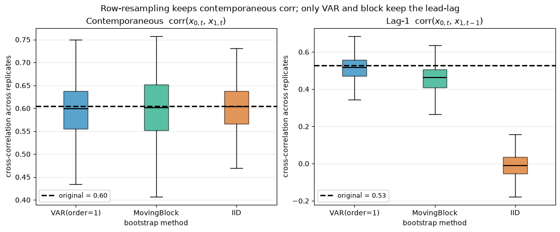
It is tempting to conclude that any row-resampler is fine for multivariate data. For the contemporaneous correlation that holds: even plain IID resampling keeps it, because it never splits a row. But IID shuffles rows independently, so it destroys every relationship that spans more than one time step, including the lead-lag cross-correlation. That gap is the reason to reach for a time-series method on multivariate data instead of a plain resampler.

from tsbootstrap import IID

methods = {
    "VAR(order=1)": ResidualBootstrap(model=VAR(order=1)),
    "MovingBlock": MovingBlock(block_length="auto"),
    "IID": IID(),
}

contemp_by_method, lag1_by_method = {}, {}
for name, spec in methods.items():
    vals = bootstrap(X, method=spec, n_bootstraps=500, random_state=0).values()
    contemp_by_method[name] = np.array([contemp_cross_corr(v) for v in vals])
    lag1_by_method[name] = np.array([lag1_cross_corr(v) for v in vals])

names = list(methods)
# Colorblind-friendly per-method colors (Okabe-Ito subset).
method_colors = {"VAR(order=1)": "#0072B2", "MovingBlock": "#009E73", "IID": "#D55E00"}

fig, axes = plt.subplots(1, 2, figsize=(11, 4.5), constrained_layout=True)
for ax, data, orig, title in [
    (axes[0], contemp_by_method, orig_contemp, "Contemporaneous  corr($x_{0,t}$, $x_{1,t}$)"),
    (axes[1], lag1_by_method, orig_lag1, "Lag-1  corr($x_{0,t}$, $x_{1,t-1}$)"),
]:
    bp = ax.boxplot(
        [data[k] for k in names],
        tick_labels=names,
        showfliers=False,
        patch_artist=True,
        medianprops={"color": "black", "lw": 1.5},
    )
    for patch, name in zip(bp["boxes"], names):
        patch.set_facecolor(method_colors[name])
        patch.set_alpha(0.65)
    ax.axhline(orig, color="black", lw=2, ls="--", label=f"original = {orig:.2f}")
    ax.set_title(title)
    ax.set_xlabel("bootstrap method")
    ax.set_ylabel("cross-correlation across replicates")
    ax.grid(True, axis="y", alpha=0.3)
    ax.legend(loc="lower left", fontsize=9, framealpha=0.9)
fig.suptitle(
    "Row-resampling keeps contemporaneous corr; only VAR and block keep the lead-lag",
    fontsize=12,
)
plt.show()

print(f"{'method':14s} {'contemp mean':>13s} {'lag-1 mean':>11s}")
for name in names:
    print(f"{name:14s} {contemp_by_method[name].mean():13.3f} {lag1_by_method[name].mean():11.3f}")
print(f"original       {orig_contemp:13.3f} {orig_lag1:11.3f}")

method          contemp mean  lag-1 mean
VAR(order=1)           0.595       0.515
MovingBlock            0.598       0.458
IID                    0.601      -0.009
original               0.604       0.528

The left panel is flat: all three methods land on the original contemporaneous correlation, because none of them splits a row. The right panel separates them. VAR and the moving block sit on the dashed lead-lag truth; IID collapses to zero. IID has thrown away the dynamic cross-dependence while keeping the static one, the kind of silent failure to watch for.

A real macro example

We repeat the check on a small macro subset from statsmodels: real GDP, real consumption, and the CPI (quarterly US data). The levels trend upward and are non-stationary, so we work with quarterly log growth rates, which a VAR can fit sensibly. The truth is no longer known, but we can still confirm that the replicate cross-correlations track the observed ones.

import pandas as pd
import statsmodels.api as sm

macro = sm.datasets.macrodata.load_pandas().data
levels = macro[["realgdp", "realcons", "cpi"]].to_numpy()
labels = ["realgdp", "realcons", "cpi"]

# Quarterly log growth (in percent): a stationary multivariate series.
growth = np.diff(np.log(levels), axis=0) * 100.0
print("growth shape:", growth.shape, " (n, d)")

orig_corr = np.corrcoef(growth.T)
print("original cross-correlation matrix:")
pd.DataFrame(orig_corr, index=labels, columns=labels).round(3)

growth shape: (202, 3)  (n, d)
original cross-correlation matrix:

	realgdp	realcons	cpi
realgdp	1.000	0.658	-0.059
realcons	0.658	1.000	-0.171
cpi	-0.059	-0.171	1.000

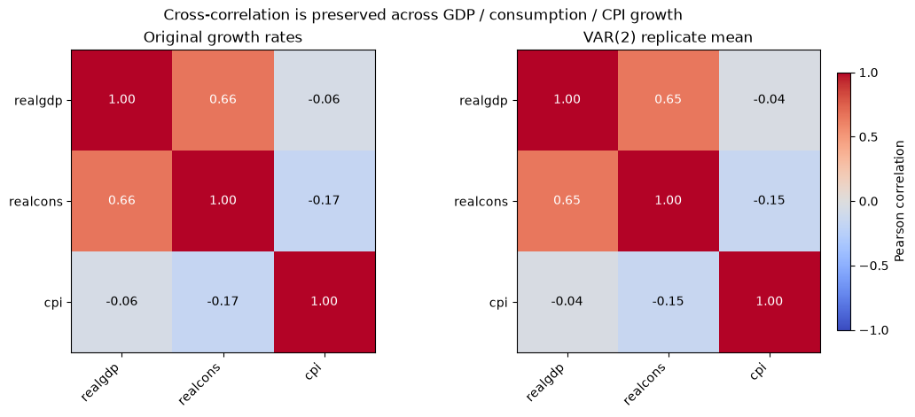
We fit a VAR(2) on the growth rates, average the replicate correlation matrices, and compare them against the original. The two matrices appear side by side as heatmaps, with the off-diagonal pairs collected into a table below.

import pandas as pd

macro_res = bootstrap(
    growth,
    method=ResidualBootstrap(model=VAR(order=2)),
    n_bootstraps=500,
    random_state=0,
)
macro_corr = np.mean([np.corrcoef(v.T) for v in macro_res.values()], axis=0)

fig, axes = plt.subplots(1, 2, figsize=(11, 4.6), constrained_layout=True)
for ax, mat, title in [
    (axes[0], orig_corr, "Original growth rates"),
    (axes[1], macro_corr, "VAR(2) replicate mean"),
]:
    im = ax.imshow(mat, vmin=-1, vmax=1, cmap="coolwarm")
    ax.set_xticks(range(len(labels)))
    ax.set_xticklabels(labels, rotation=45, ha="right")
    ax.set_yticks(range(len(labels)))
    ax.set_yticklabels(labels)
    ax.set_title(title)
    # Annotate each cell; pick black or white text for contrast against the fill.
    for i in range(len(labels)):
        for j in range(len(labels)):
            val = mat[i, j]
            ax.text(
                j,
                i,
                f"{val:.2f}",
                ha="center",
                va="center",
                fontsize=10,
                color="white" if abs(val) > 0.6 else "black",
            )
cbar = fig.colorbar(im, ax=axes, shrink=0.85, pad=0.02)
cbar.set_label("Pearson correlation")
cbar.set_ticks([-1.0, -0.5, 0.0, 0.5, 1.0])
fig.suptitle(
    "Cross-correlation is preserved across GDP / consumption / CPI growth",
    fontsize=12,
)
plt.show()

# Off-diagonal pairs side by side: original vs replicate mean.
pairs = [(0, 1), (0, 2), (1, 2)]
comparison = pd.DataFrame(
    {
        "pair": [f"{labels[i]} / {labels[j]}" for i, j in pairs],
        "original": [orig_corr[i, j] for i, j in pairs],
        "VAR(2) replicate mean": [macro_corr[i, j] for i, j in pairs],
    }
)
comparison["difference"] = comparison["VAR(2) replicate mean"] - comparison["original"]
comparison.round(3)

	pair	original	VAR(2) replicate mean	difference
0	realgdp / realcons	0.658	0.652	-0.006
1	realgdp / cpi	-0.059	-0.041	0.018
2	realcons / cpi	-0.171	-0.149	0.022

The two heatmaps match: the strong GDP-consumption co-movement and the weak, slightly negative links to CPI growth all carry over into the VAR replicates. The bootstrap has preserved the joint structure of the real series, not just the marginals.

diagnose() on multivariate input

diagnose() inspects the series and recommends method specifications. When it sees more than one column it adds a VAR-based recommendation, because a VAR is the model-based way to capture cross-series dependence, while noting that block methods preserve it by resampling whole rows. We run it on both the non-stationary levels and the stationary growth rates.

from tsbootstrap import diagnose

for name, series in [("macro levels", levels), ("macro growth", growth)]:
    d = diagnose(series)
    print(f"{name} (n_series={d.n_series}):")
    print(f"  recommended: {d.recommended_methods}")
    for note in d.notes:
        print(f"  - {note}")
    print()

macro levels (n_series=3):
  recommended: ('ResidualBootstrap(model=VAR(...))', 'ResidualBootstrap(model=ARIMA(...))', 'SieveAR')
  - Series looks non-stationary (unit root): difference it via ARIMA, or use the sieve.
  - Multivariate input: VAR captures cross-series dependence; block methods preserve it by resampling whole rows.

macro growth (n_series=3):
  recommended: ('ResidualBootstrap(model=VAR(...))', 'StationaryBlock', 'MovingBlock', 'SieveAR')
  - Serial dependence present (lag-1 autocorrelation 0.64): use a block method or the sieve.
  - Multivariate input: VAR captures cross-series dependence; block methods preserve it by resampling whole rows.
  - Suggested automatic block length (Politis-White): 20.

For both the levels and the growth rates, diagnose() puts ResidualBootstrap(model=VAR(...)) first, because the input is multivariate. The rest of the recommendation reflects what else it measured: an integrated model for the trending levels (a unit root), block methods and the sieve for the stationary growth rates. The multivariate signal is detected from the column count alone, so it fires regardless of the stationarity verdict.

Choosing for multivariate input

Multivariate data is defined by how its series move together, so a bootstrap must preserve that joint structure. Row-resampling methods (the block family) keep it by copying whole rows of (n, d) input, which is robust and model-free. ResidualBootstrap(model=VAR(...)) keeps it by fitting and replaying the vector dynamics, which additionally captures lead-lag relationships that a single-step resampler cannot. Plain IID keeps the contemporaneous correlation but discards the dynamics, so on data with real lead-lag structure a time-series method earns its keep. diagnose() flags the multivariate case for you and points at the VAR.