Run this tutorial: Open in Colab | Launch Binder

Reproducibility and memory-bounded scaling

If you cannot reproduce a bootstrap result, you cannot cite it. tsbootstrap answers that on two fronts: a run is deterministic for a fixed seed and environment, and it records its own provenance. From there we scale to a large number of replicates without running out of memory, using bootstrap_reduce, which keeps only a per-replicate statistic instead of the full array of resampled series.

Throughout we simulate a stationary AR(1), x[t] = phi * x[t-1] + e[t].

# On Colab or Binder, install tsbootstrap first (skipped if already present):
try:
    import tsbootstrap  # noqa: F401
except ImportError:
    %pip install -q "tsbootstrap[examples]"

A small AR(1) series

A stationary AR(1) with phi = 0.6 and unit-variance Gaussian noise. We keep n small; the scaling demo later pushes the number of replicates, not the series length.

import matplotlib.pyplot as plt
import numpy as np

PHI = 0.6


def ar1(n, phi=PHI, rng=None):
    """Stationary AR(1) with unit-variance Gaussian noise, started at 0."""
    rng = np.random.default_rng() if rng is None else rng
    x = np.zeros(n)
    e = rng.standard_normal(n)
    for t in range(1, n):
        x[t] = phi * x[t - 1] + e[t]
    return x


n = 120
x = ar1(n, PHI, np.random.default_rng(0))
x[:5]

array([ 0.        , -0.13210486,  0.56115973,  0.44159596, -0.2707118 ])

Reproducibility: same seed, identical results

Pass an integer random_state and two runs return bitwise-identical arrays. The RNG contract is per-replicate: replicate i is bound to its own generator, derived from SeedSequence.spawn(n)[i], before any work is dispatched. Because the stream for sample i is fixed before parallelisation, the results are invariant to the worker count and to how the replicates are chunked. We verify exact equality with np.array_equal.

from tsbootstrap import MovingBlock, bootstrap

run_a = bootstrap(x, method=MovingBlock(block_length=10), n_bootstraps=200, random_state=0)
run_b = bootstrap(x, method=MovingBlock(block_length=10), n_bootstraps=200, random_state=0)

values_equal = np.array_equal(run_a.values(), run_b.values())
indices_equal = np.array_equal(run_a.indices(), run_b.indices())
print(f"values identical across two random_state=0 runs: {values_equal}")
print(f"indices identical across two random_state=0 runs: {indices_equal}")

# A different seed gives a different draw (sanity check that the seed is doing something).
run_c = bootstrap(x, method=MovingBlock(block_length=10), n_bootstraps=200, random_state=1)
print(
    f"random_state=1 differs from random_state=0: {not np.array_equal(run_a.values(), run_c.values())}"
)

values identical across two random_state=0 runs: True
indices identical across two random_state=0 runs: True
random_state=1 differs from random_state=0: True

random_state accepts an int, a NumPy Generator, a SeedSequence, or None. An int (or a SeedSequence) gives a reproducible run for any worker count. A Generator is consumed once: a 128-bit seed is drawn from it and recorded, so the live generator is never shared across processes, yet the run is reproducible from the recorded entropy. None uses OS entropy (non-reproducible), but the drawn entropy is still recorded for provenance. The next cell shows where that recorded entropy lives.

Worker-count invariance is the same contract NumPy and scikit-learn give: results are reproducible for a fixed seed and environment (OS, hardware, BLAS, NumPy version).

Provenance: the run records how it was produced

Every result carries a BootstrapRunMetadata record at result.metadata, which holds what you need to reproduce or cite the run. The next cell prints its fields, so what you read is what the dataclass stores.

import pandas as pd

meta = run_a.metadata
provenance = pd.DataFrame(
    [
        ("method", repr(meta.method)),
        ("method_params", meta.method_params),
        ("n_bootstraps", meta.n_bootstraps),
        ("n_obs", meta.n_obs),
        ("n_series", meta.n_series),
        ("random_state_kind", repr(meta.random_state_kind)),
        ("seed_entropy", meta.seed_entropy),
        ("backend", repr(meta.backend)),
        ("versions", meta.versions),
        ("references", meta.references),
        ("warnings", meta.warnings),
        ("failed", meta.failed),
        ("failure_reason", repr(meta.failure_reason)),
    ],
    columns=["field", "value"],
).set_index("field")
provenance

	value
field
method	'moving_block'
method_params	{'kind': 'moving_block', 'block_length': 10}
n_bootstraps	200
n_obs	120
n_series	1
random_state_kind	'int'
seed_entropy	0
backend	None
versions	{'numpy': '2.4.6', 'scipy': '1.15.3', 'tsboots...
references	(Kunsch 1989, Liu-Singh 1992)
warnings	()
failed	False
failure_reason	None

Two fields carry the provenance that matters most. random_state_kind records how the seed was supplied (here 'int'), and seed_entropy is the actual entropy the run consumed. Even with random_state=None the seed_entropy is populated, so an exploratory run can be replayed exactly by feeding its recorded entropy back in. references lists the method’s literature citations, and versions pins the library versions, so a result is self-documenting for a paper or report.

# The recorded entropy replays a 'random' run exactly.
auto = bootstrap(x, method=MovingBlock(block_length=10), n_bootstraps=50, random_state=None)
recorded = auto.metadata.seed_entropy
print(f"random_state_kind: {auto.metadata.random_state_kind!r}")
print(f"recorded seed_entropy: {recorded}")

replay = bootstrap(
    x,
    method=MovingBlock(block_length=10),
    n_bootstraps=50,
    random_state=np.random.SeedSequence(recorded),
)
print(
    f"replay from recorded entropy reproduces the run: {np.array_equal(auto.values(), replay.values())}"
)

random_state_kind: 'none'
recorded seed_entropy: 278104144765395418338305278694271410265
replay from recorded entropy reproduces the run: True

Memory-bounded scaling to large B

Conformal and UQ calibration want many replicates. But the full result is a (B, n) array: at B = 5000 and even a modest n that materialised array can be large, and for longer series it stops fitting in RAM. bootstrap_reduce solves this by applying a statistic to each replicate inside the same chunked loop bootstrap uses, keeping only the (B, |theta|) array of statistic values. Peak memory is O(B * |theta|) instead of O(B * n).

The statistic is a callable (values, indices) -> scalar | array. values is one replicate of shape (n,); indices is its original-observation indices (or None for recursive methods). It must be independent across replicates, since it is evaluated one replicate at a time. We use a cheap statistic, the mean of the replicate, so B = 5000 runs fast.

from tsbootstrap import bootstrap_reduce


def replicate_mean(values, indices):
    """Cheap per-replicate statistic: the sample mean. indices is unused here."""
    return values.mean()


B_large = 5000
reduced = bootstrap_reduce(
    x,
    method=MovingBlock(block_length=10),
    statistic=replicate_mean,
    n_bootstraps=B_large,
    random_state=0,
)

print(f"reduced.statistics shape: {reduced.statistics.shape}   # (B, |theta|)")
print(f"number of replicates kept: {len(reduced)}")
print(f"reduced.failed: {reduced.failed}")

reduced.statistics shape: (5000,)   # (B, |theta|)
number of replicates kept: 5000
reduced.failed: False

A confidence interval without the full array

ReducedResult.quantile([...]) takes exact quantiles over the B replicates. A percentile confidence interval for the mean falls straight out, computed from the 5000-row statistic array, never from a materialised (5000, 120) array of series.

lo, hi = reduced.quantile([0.025, 0.975])
point = float(np.median(reduced.statistics))
print(f"95% percentile CI for the mean (B={B_large}): [{lo:.4f}, {hi:.4f}]")
print(f"interval width: {hi - lo:.4f}")
print(f"observed sample mean: {x.mean():.4f}")

95% percentile CI for the mean (B=5000): [-0.2740, 0.5846]
interval width: 0.8586
observed sample mean: 0.1730

Conceptual memory contrast

The two paths keep different things in memory. The full path holds the resampled series; the reduced path holds only the statistic. For a scalar statistic like the mean, |theta| = 1, so the reduced footprint is the series length n times smaller than the full one. The numbers below are the array sizes the two paths would hold at B = 5000; only the reduced one was actually materialised here.

bytes_per_float = 8
full_floats = B_large * n  # O(B * n): the materialised (B, n) array
reduced_floats = B_large * 1  # O(B * |theta|): one statistic per replicate

memory = pd.DataFrame(
    {
        "array shape": [f"(B, n) = ({B_large}, {n})", f"(B, 1) = ({B_large}, 1)"],
        "floats held": [full_floats, reduced_floats],
        "size (MB)": [full_floats * bytes_per_float / 1e6, reduced_floats * bytes_per_float / 1e6],
    },
    index=["full path", "reduced path"],
)
print(f"reduction factor: {full_floats / reduced_floats:.0f}x  (equal to the series length n)")
memory

reduction factor: 120x  (equal to the series length n)

	array shape	floats held	size (MB)
full path	(B, n) = (5000, 120)	600000	4.80
reduced path	(B, 1) = (5000, 1)	5000	0.04

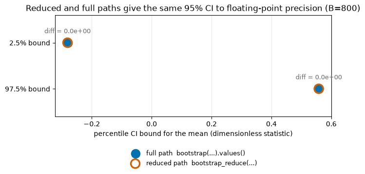
The reduced CI matches the full-array CI

Reducing on the fly gives the same answer as keeping the full array. At a smaller B where the full array is cheap, we compute the same percentile CI both ways: once from the full bootstrap(...).values() array, once from bootstrap_reduce(...). With the same seed and method the replicates are identical, so the intervals agree to floating-point precision.

B_check = 800
common = {"method": MovingBlock(block_length=10), "n_bootstraps": B_check, "random_state": 0}

# Full path: materialise every series, then take the per-replicate mean.
full = bootstrap(x, **common)
full_means = full.values().mean(axis=1)
full_lo, full_hi = np.quantile(full_means, [0.025, 0.975])

# Reduced path: never materialise the (B, n) array.
red = bootstrap_reduce(x, statistic=replicate_mean, **common)
red_lo, red_hi = red.quantile([0.025, 0.975])

comparison = pd.DataFrame(
    {
        "2.5% bound": [full_lo, float(red_lo), abs(full_lo - float(red_lo))],
        "97.5% bound": [full_hi, float(red_hi), abs(full_hi - float(red_hi))],
    },
    index=["full path", "reduced path", "abs. difference"],
)
print(f"CI bounds identical to floating point: {np.allclose([full_lo, full_hi], [red_lo, red_hi])}")
print(f"per-replicate means identical:         {np.allclose(full_means, red.statistics.ravel())}")
comparison

CI bounds identical to floating point: True
per-replicate means identical:         True

	2.5% bound	97.5% bound
full path	-0.281177	0.558246
reduced path	-0.281177	0.558246
abs. difference	0.000000	0.000000

# The two CIs land on top of each other: full path (markers) vs reduced path (open rings).
fig, ax = plt.subplots(figsize=(7, 3.2), layout="constrained")

bounds = ["2.5% bound", "97.5% bound"]
ypos = [1, 0]  # draw 2.5% on top, 97.5% below, so the two rows read cleanly
full_vals = [full_lo, full_hi]
red_vals = [float(red_lo), float(red_hi)]

ax.scatter(
    full_vals,
    ypos,
    s=170,
    color="#0072B2",
    marker="o",
    label="full path  bootstrap(...).values()",
    zorder=3,
)
ax.scatter(
    red_vals,
    ypos,
    s=170,
    facecolors="none",
    edgecolors="#D55E00",
    linewidths=2.4,
    marker="o",
    label="reduced path  bootstrap_reduce(...)",
    zorder=4,
)

for y, fv, rv in zip(ypos, full_vals, red_vals):
    ax.annotate(
        f"diff = {abs(fv - rv):.1e}",
        xy=(fv, y),
        xytext=(0, 14),
        textcoords="offset points",
        ha="center",
        fontsize=9,
        color="dimgray",
    )

ax.set_yticks(ypos)
ax.set_yticklabels(bounds)
ax.set_ylim(-0.6, 1.6)
ax.set_xlabel("percentile CI bound for the mean (dimensionless statistic)")
ax.set_title("Reduced and full paths give the same 95% CI to floating-point precision (B=800)")
ax.legend(loc="lower center", bbox_to_anchor=(0.5, -0.55), ncol=1, frameon=False, fontsize=9)
ax.grid(axis="x", alpha=0.3)
plt.show()

Putting it together

One figure ties the two ideas together. We grow B and watch the reduced-path percentile CI for the mean settle as more replicates accumulate, with the large-B interval drawn as a band. Each point reuses the same seed, so the curve is itself reproducible.

grid = [50, 100, 200, 500, 1000, 2000, 5000]
los, his = [], []
for b in grid:
    r = bootstrap_reduce(
        x,
        method=MovingBlock(block_length=10),
        statistic=replicate_mean,
        n_bootstraps=b,
        random_state=0,
    )
    lo_b, hi_b = r.quantile([0.025, 0.975])
    los.append(float(lo_b))
    his.append(float(hi_b))

los = np.asarray(los)
his = np.asarray(his)

fig, ax = plt.subplots(figsize=(8, 4.5), layout="constrained")

# Reference band: the large-B interval the curves are converging toward.
ax.axhspan(
    lo, hi, color="#56B4E9", alpha=0.22, zorder=0, label=f"reference interval at B={B_large}"
)

# The reduced-path CI bounds as they accumulate replicates.
ax.plot(
    grid, los, "o-", color="#0072B2", lw=2, markersize=7, label="2.5% quantile (lower CI bound)"
)
ax.plot(
    grid, his, "s--", color="#D55E00", lw=2, markersize=7, label="97.5% quantile (upper CI bound)"
)
ax.axhline(
    x.mean(),
    color="black",
    lw=1.4,
    ls=":",
    zorder=2,
    label=f"observed sample mean = {x.mean():.3f}",
)

ax.set_xscale("log")
ax.set_xticks(grid)
ax.set_xticklabels(grid)
ax.set_xlabel("number of bootstrap replicates B (log scale)")
ax.set_ylabel("percentile CI bound for the mean\n(dimensionless statistic)")
ax.set_title("Reduced-path 95% CI converges to its large-B value as B grows")
ax.legend(loc="center right", fontsize=9, framealpha=0.92)
ax.grid(alpha=0.3)
plt.show()

print(f"CI at B={grid[0]:>4d}: [{los[0]:.4f}, {his[0]:.4f}]  width {his[0] - los[0]:.4f}")
print(f"CI at B={grid[-1]:>4d}: [{los[-1]:.4f}, {his[-1]:.4f}]  width {his[-1] - los[-1]:.4f}")

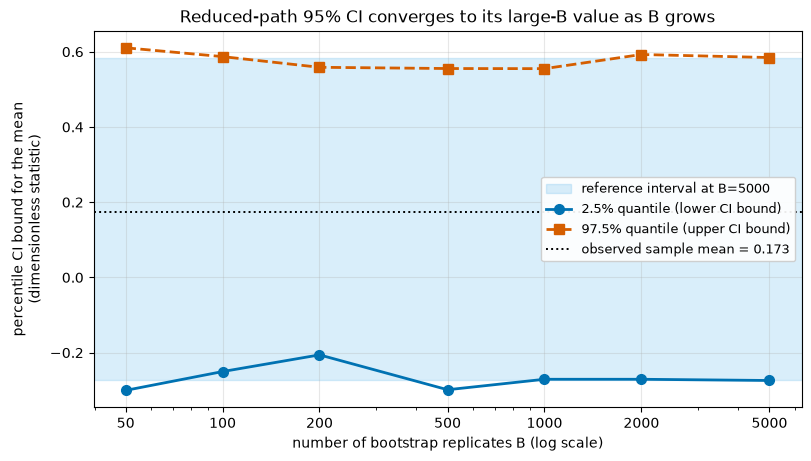
CI at B=  50: [-0.3003, 0.6105]  width 0.9108
CI at B=5000: [-0.2740, 0.5846]  width 0.8586

Closing the loop on reproducibility

A fixed integer seed gives bitwise-identical results no matter how the work is parallelised. Every run records the entropy and the library versions needed to replay or cite it. And bootstrap_reduce scales the replicate count to whatever your calibration needs without holding the full (B, n) array in memory, while returning the same quantiles the full array would.