Run this tutorial: Open in Colab | Launch Binder

Model-based bootstraps: residual and sieve

Block bootstraps keep dependence by resampling contiguous chunks of the observed series. Model-based bootstraps work differently. They fit one parametric model to the data, then regenerate each replicate recursively from the fitted dynamics driven by resampled, centered innovations:

x*[t] = c + sum_j phi_j x*[t-j] + e*[t]

Nothing is resampled at the level of observations. A replicate is a new path simulated forward through the estimated dynamics, so there are no observation indices and no out-of-bag set. There are three model-based specs in tsbootstrap to work through:

1. ResidualBootstrap(model=AR(order=...)) on a synthetic AR(2).

2. ResidualBootstrap(model=ARIMA(order=(p, d, q))) on a near-unit-root real series that needs differencing.

3. SieveAR, which picks the AR order from the data before resampling.

We close on the stability guard: what tsbootstrap does when the fitted model is explosive or sits on a unit root. The code runs offline against bundled datasets.

# On Colab or Binder, install tsbootstrap first (skipped if already present):
try:
    import tsbootstrap  # noqa: F401
except ImportError:
    %pip install -q "tsbootstrap[examples]"

# The ARIMA and sieve paths use statsmodels, which ships in the [examples] extra
# (it pulls in tsbootstrap[models]). The bundled datasets come from sktime and
# statsmodels, both also in [examples].

A synthetic AR(2)

We start with a stationary AR(2) so the dependence structure is known exactly: x[t] = 0.5 x[t-1] + 0.3 x[t-2] + e[t]. The two coefficients sum to 0.8, well inside the stationary region, so the fitted model will be stable.

import matplotlib.pyplot as plt
import numpy as np

from tsbootstrap import AR, ARIMA, ResidualBootstrap, SieveAR, bootstrap

rng = np.random.default_rng(0)
n = 300
phi1, phi2 = 0.5, 0.3
x = np.zeros(n)
e = rng.standard_normal(n)
for t in range(2, n):
    x[t] = phi1 * x[t - 1] + phi2 * x[t - 2] + e[t]
x[:5]

array([ 0.        ,  0.        ,  0.64042265,  0.42511144, -0.13098686])

ResidualBootstrap with a fixed-order AR

ResidualBootstrap(model=AR(order=2)) fits an AR(2) once by ordinary least squares, centers its residuals, and then simulates each replicate forward. The innovation resampler defaults to IID(): the centered residuals are drawn with replacement, independently, and fed through the fitted recursion. The result has the same (n_bootstraps, n) shape as a block bootstrap, but every row is a fresh simulated path rather than a reshuffling of the original points.

res_ar = bootstrap(x, method=ResidualBootstrap(model=AR(order=2)), n_bootstraps=200, random_state=1)
samples_ar = res_ar.values()
samples_ar.shape  # (n_bootstraps, n)

(200, 300)

No observation indices, no out-of-bag

This is the structural difference from block and IID methods. Because a recursive replicate is simulated rather than resampled, there is no mapping back to original observation positions. indices() returns None, and asking for the out-of-bag mask raises rather than inventing one. The EnbPI uncertainty layer, which is built on the out-of-bag structure, therefore cannot consume a recursive method.

from tsbootstrap.errors import OOBUnavailableError

print("indices():", res_ar.indices())  # None for a recursive method

try:
    res_ar.get_oob_mask()
except OOBUnavailableError as exc:
    print("get_oob_mask() raised:", type(exc).__name__)
    print(str(exc).splitlines()[0])

indices(): None
get_oob_mask() raised: OOBUnavailableError
[TSB_OOB_UNAVAILABLE] in-bag/out-of-bag counts require observation indices, which method 'residual' does not produce Hint: Use an observation-resampling method (IID or a block method) for OOB.

Replicate paths

Each replicate is a new realisation of the same fitted AR(2) dynamics. They share the persistence and variance of the original but are not reshufflings of it: the recursion can wander anywhere the model allows.

from matplotlib.lines import Line2D

fig, ax = plt.subplots(figsize=(9, 3.8), layout="constrained")
for i in range(6):
    ax.plot(samples_ar[i], color="tab:blue", alpha=0.45, lw=1.0)
ax.plot(x, color="black", lw=2.0, label="original series")
# Proxy handle so the replicate cloud gets one legend entry rather than six.
replicate_handle = Line2D([], [], color="tab:blue", alpha=0.7, lw=1.0)
ax.set_title("AR(2): original series vs 6 residual-bootstrap replicate paths")
ax.set_xlabel("time index t")
ax.set_ylabel("x[t] (value)")
ax.legend(
    handles=[ax.lines[-1], replicate_handle],
    labels=["original series", "bootstrap replicates (n=6)"],
    loc="upper right",
)
plt.show()

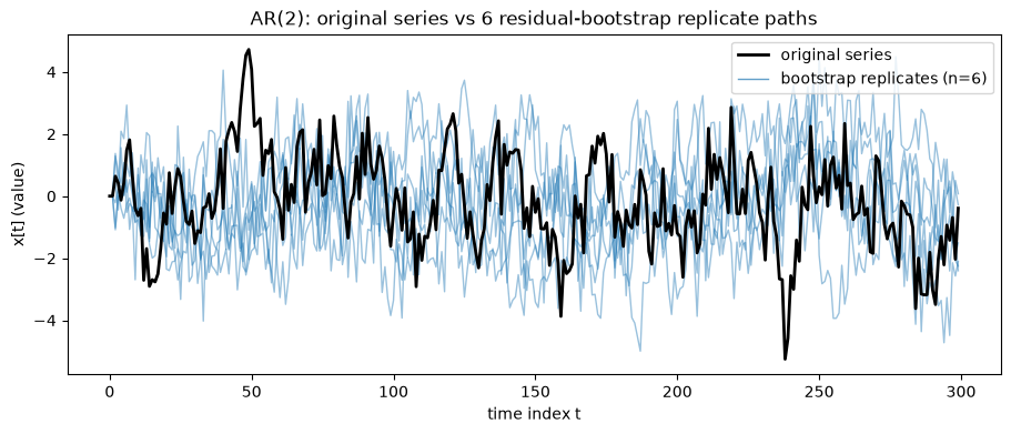
A quick sanity check that the resampling is innovation-based. The original series and the replicates have comparable lag-1 autocorrelation, because every replicate is driven through the same fitted recursion. Plain IID resampling of the observations would instead collapse that autocorrelation toward zero.

import pandas as pd


def lag1_acf(series):
    s = np.asarray(series, dtype=float)
    s = s - s.mean()
    return float(np.dot(s[:-1], s[1:]) / np.dot(s, s))


rep_acf = np.array([lag1_acf(v) for v in samples_ar])
acf_table = pd.DataFrame(
    {"lag-1 ACF": [lag1_acf(x), rep_acf.mean()]},
    index=["original series", "replicate mean (n=200)"],
)
acf_table.round(3)

	lag-1 ACF
original series	0.72
replicate mean (n=200)	0.70

ResidualBootstrap with ARIMA on a near-unit-root series

A pure AR cannot represent a series with a stochastic trend. The Nile river annual flow (statsmodels’ bundled nile dataset, 100 yearly observations) drifts like a near-unit-root process: its level wanders rather than reverting to a fixed mean. The integrated ARIMA(order=(p, d, q)) model handles this by differencing d times before fitting an ARMA to the stationary differenced series, then integrating each simulated path back up to the level.

ARIMA needs the MA / maximum-likelihood machinery in statsmodels, which is the [models] extra (included in [examples]). AR, VAR, and the sieve are fit by direct OLS and need no optional dependency.

import statsmodels.api as sm

nile = sm.datasets.nile.load_pandas().data["volume"].to_numpy(dtype=float)
print("nile length:", nile.shape[0])

res_arima = bootstrap(
    nile,
    method=ResidualBootstrap(model=ARIMA(order=(1, 1, 1))),
    n_bootstraps=200,
    random_state=2,
)
samples_arima = res_arima.values()
print("ARIMA replicate shape:", samples_arima.shape)
print("run failed:", res_arima.metadata.failed)
print("indices():", res_arima.indices())  # still None: ARIMA is recursive too

nile length: 100
ARIMA replicate shape: (200, 100)
run failed: False
indices(): None

fig, ax = plt.subplots(figsize=(9, 3.8), layout="constrained")
for i in range(6):
    ax.plot(samples_arima[i], color="tab:green", alpha=0.45, lw=1.0)
ax.plot(nile, color="black", lw=2.0, label="Nile flow")
replicate_handle = Line2D([], [], color="tab:green", alpha=0.7, lw=1.0)
ax.set_title("Nile annual flow: observed vs 6 ARIMA(1,1,1) replicate paths")
ax.set_xlabel("year index (1871 = 0)")
ax.set_ylabel("annual flow (1e8 m^3)")
ax.legend(
    handles=[ax.lines[-1], replicate_handle],
    labels=["observed Nile flow", "bootstrap replicates (n=6)"],
    loc="upper right",
)
plt.show()

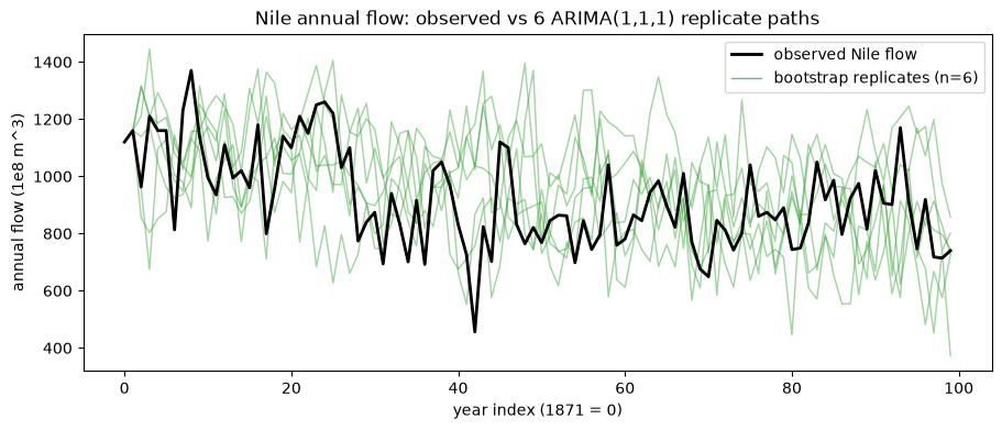
The replicates condition on the observed initial differenced state, so they start at the right level and then diverge as the resampled innovations propagate. The d = 1 differencing is what lets a model-based bootstrap follow a wandering level that a stationary AR could not.

SieveAR: let the data choose the order

The sieve bootstrap is a residual AR bootstrap that does not ask you to fix the order. SieveAR selects the AR order once from the data by an information criterion (default bic, with aic and hqic available), bounded by min_lag and max_lag, then runs the recursive AR residual bootstrap at that order.

We use the bundled sunspot series (statsmodels’ sunspots, 309 yearly counts), which has rich autoregressive structure. The order chosen is the same one SieveAR uses internally; select_ar_order is the function the spec calls.

import pandas as pd

from tsbootstrap.model.fit import select_ar_order

sun = sm.datasets.sunspots.load_pandas().data["SUNACTIVITY"].to_numpy(dtype=float)
print("sunspots length:", sun.shape[0])

order_table = pd.DataFrame(
    {
        "criterion": ["bic", "aic", "hqic"],
        "selected_AR_order": [
            select_ar_order(sun, criterion="bic"),
            select_ar_order(sun, criterion="aic"),
            select_ar_order(sun, criterion="hqic"),
        ],
    }
).set_index("criterion")
order_bic = int(order_table.loc["bic", "selected_AR_order"])
order_table

sunspots length: 309

	selected_AR_order
criterion
bic	9
aic	9
hqic	9

res_sieve = bootstrap(sun, method=SieveAR(criterion="bic"), n_bootstraps=200, random_state=3)
samples_sieve = res_sieve.values()
print("sieve replicate shape:", samples_sieve.shape)
print("indices():", res_sieve.indices())  # recursive: None

fig, ax = plt.subplots(figsize=(9, 3.8), layout="constrained")
for i in range(6):
    ax.plot(samples_sieve[i], color="tab:purple", alpha=0.40, lw=1.0)
ax.plot(sun, color="black", lw=2.0, label="sunspots")
replicate_handle = Line2D([], [], color="tab:purple", alpha=0.7, lw=1.0)
ax.set_title(f"Sunspots: observed vs 6 SieveAR replicates (selected order {order_bic})")
ax.set_xlabel("year index (1700 = 0)")
ax.set_ylabel("sunspot activity (count)")
ax.legend(
    handles=[ax.lines[-1], replicate_handle],
    labels=["observed sunspots", "bootstrap replicates (n=6)"],
    loc="upper right",
)
plt.show()

sieve replicate shape: (200, 309)
indices(): None

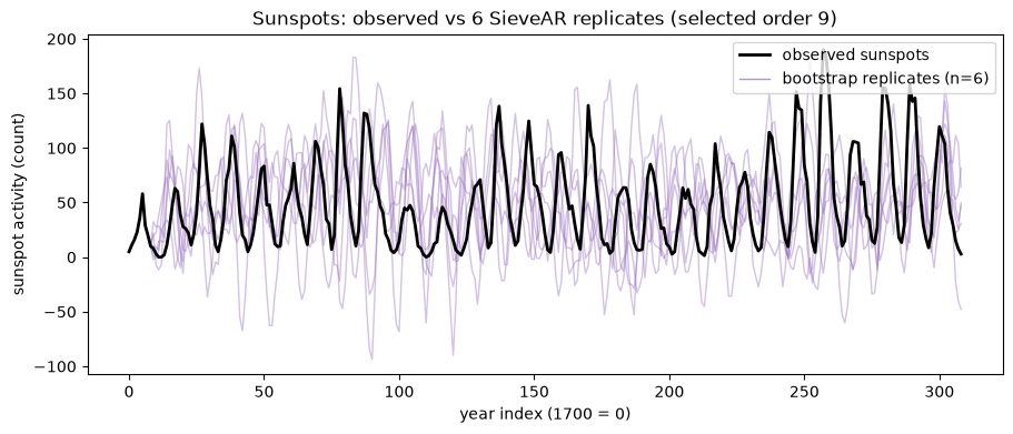
SieveAR defaults min_lag=1 and leaves max_lag=None, which lets the selector consider up to roughly 10 * log10(n) lags. Tightening the bounds, for example SieveAR(min_lag=1, max_lag=4), caps the search and would force a smaller order here.

The stability guard

A recursive bootstrap of a non-stationary fitted model produces explosive paths, so tsbootstrap checks the fitted dynamics before simulating. The check is on the companion-matrix spectral radius of the fitted AR coefficients:

• radius >= 1.0: the model is non-stationary. The behaviour depends on stability_policy (a field on every model spec, default "raise").

• 0.98 <= radius < 1.0: near a unit root. The run proceeds but emits a NearUnitRootWarning.

Near a unit root: warn, but proceed

A random walk has no mean reversion, so a fitted AR(1) lands just below 1; the longer the walk, the closer the fitted coefficient sits to 1. The bootstrap runs and returns replicates, but warns that the paths may be unreliable.

import warnings

from tsbootstrap.errors import ModelStabilityError, NearUnitRootWarning

# A longer random walk pins the fitted AR(1) coefficient into the [0.98, 1.0) band.
rw = np.cumsum(np.random.default_rng(0).standard_normal(600))

with warnings.catch_warnings(record=True) as caught:
    warnings.simplefilter("always")
    res_rw = bootstrap(
        rw, method=ResidualBootstrap(model=AR(order=1)), n_bootstraps=50, random_state=4
    )
near_unit = [w for w in caught if issubclass(w.category, NearUnitRootWarning)]
print("replicates produced:", len(res_rw))
print("run failed:", res_rw.metadata.failed)
print("NearUnitRootWarning emitted:", bool(near_unit))
if near_unit:
    print(str(near_unit[0].message).splitlines()[0])

replicates produced: 50
run failed: False
NearUnitRootWarning emitted: True
[TSB_NEAR_UNIT_ROOT] fitted AR model is near a unit root (companion spectral radius 0.9935); bootstrap paths may be unreliable

Explosive fit: raise, or skip

For a genuinely explosive process the fitted coefficient exceeds 1 and the spectral radius crosses the threshold. We build a deterministic explosive series (z[t] = 1.05 z[t-1] + small noise) so the fitted AR(1) is clearly non-stationary.

With the default stability_policy="raise", the run raises ModelStabilityError rather than returning explosive garbage.

explosive = np.empty(200)
explosive[0] = 1.0
for t in range(1, explosive.shape[0]):
    explosive[t] = 1.05 * explosive[t - 1] + 0.01 * rng.standard_normal()

try:
    bootstrap(
        explosive,
        method=ResidualBootstrap(model=AR(order=1)),  # stability_policy="raise" default
        n_bootstraps=10,
        random_state=5,
    )
except ModelStabilityError as exc:
    print("raised:", type(exc).__name__)
    print(str(exc).splitlines()[0])

raised: ModelStabilityError
[TSB_UNSTABLE_MODEL] fitted AR model is non-stationary (companion spectral radius 1.0500 >= 1); a recursive bootstrap would produce explosive paths

Setting stability_policy="skip" turns that hard failure into an empty result instead. The whole run fails as a unit: no replicates are generated, len(result) is 0, and the metadata records the failure with a reason. The run never falls back to a different method silently. A batch caller can detect the empty result and route around it.

res_skip = bootstrap(
    explosive,
    method=ResidualBootstrap(model=AR(order=1, stability_policy="skip")),
    n_bootstraps=10,
    random_state=5,
)
print("number of replicates:", len(res_skip))
print("values() shape:", res_skip.values().shape)
print("metadata.failed:", res_skip.metadata.failed)
print("failure_reason:", res_skip.metadata.failure_reason.splitlines()[0])

number of replicates: 0
values() shape: (0,)
metadata.failed: True
failure_reason: [TSB_UNSTABLE_MODEL] fitted AR model is non-stationary (companion spectral radius 1.0500 >= 1); a recursive bootstrap would produce explosive paths

The three model-based specs at a glance

Model-based bootstraps fit a parametric model once, then regenerate each replicate recursively from the fitted dynamics and resampled centered innovations:

• ResidualBootstrap(model=AR(order=p)): fixed-order AR, fit by OLS, IID innovation resampling by default.

• ResidualBootstrap(model=ARIMA(order=(p, d, q))): differences d times, fits an ARMA (needs statsmodels), integrates each simulated path back to the level. Use it for a near-unit-root or trending series.

• SieveAR: picks the AR order from the data by an information criterion, then runs the recursive AR residual bootstrap.

All three are recursive, so indices() is None and there is no out-of-bag set, which is why these methods are not EnbPI-capable. All three also refuse to simulate from an unstable fit: a near-unit-root model warns, an explosive one either raises (stability_policy="raise", the default) or returns a flagged empty result (stability_policy="skip").